Pipeline de Genómica en R

Autor/a

Francisco Ascue Orosco

Descarga de genomas desde NCBI

En esta sección, se realiza la descarga de un genoma desde la base de datos del NCBI utilizando el código proporcionado:

url <- fromJSON(file = "data/reference/ref.json")
filename <- "GCF_000085865.1_ASM8586v1_genomic.fna.gz"
download_genome(url$urlref, filename, "data/reference/")

Aclaración

El código utiliza el archivo JSON ref.json para obtener la URL del genoma y luego descarga el genoma en formato FASTA comprimido. Los archivos de genoma descargados se almacenan en el directorio data/reference/.

Descarga de archivos

En resumen

El código descarga archivos SRA utilizando los identificadores específicos proporcionados (SRR15616379 y SRR26204001) y luego los convierte en archivos FASTQ en el directorio especificado. Ver Aqui

Control de calidad de archivos FASTQ

En esta sección, se realiza un control de calidad de los archivos FASTQ descargados utilizando la biblioteca fastqc. Primero, se listan las lecturas FASTQ y se genera un perfil de calidad:

lecturas <- list_fastq(pattern = c("SRR15616379_1.fastq.gz", "SRR15616379_2.fastq.gz"))

Luego, se ejecuta fastqc para realizar un control de calidad más detallado:

library(fastqcr)
fastqc(fq.dir = "data/rawdata/", # Directorio de archivos FASTQ
       qc.dir = "results/", # Directorio de resultados
       threads = 4,
       fastqc.path = "/home/fascue/Descargas/FastQC/fastqc"
)

Este código genera informes de calidad en el directorio results/.

Filtrado de lecturas de archivos FASTQ

En esta sección, se realiza el filtrado de lecturas de los archivos FASTQ utilizando la función filter_reads previamente definida:

log_filter <- filter_reads(name = lecturas$name, lf = lecturas$lf, 
             lr = lecturas$lr, trunc = 250)

El código ejecuta la función filter_reads en las lecturas previamente listadas, aplicando un valor de truncamiento de 250. El registro del filtrado se almacena en la variable log_filter.

Ensamblaje de genomas

En esta sección, se realiza el ensamblaje de genomas utilizando la biblioteca bowtie2. Primero, se descomprime el genoma de referencia:

gunzip("data/reference/GCF_000085865.1_ASM8586v1_genomic.fna.gz")

Luego, se construye el índice de referencia para bowtie2:

bowtie2_build("data/reference/GCF_000085865.1_ASM8586v1_genomic.fna",
              bt2Index = "data/reference/index/myco" , overwrite = TRUE)

Finalmente, se realiza el alineamiento de los archivos FASTQ a la referencia utilizando bowtie2:

bowtie2(bt2Index = "data/reference/index/myco", 
        samOutput = "results/SRR15616379.sam", 
        seq1 = "data/processed_data/filtered_F/SRR15616379_filt_1.fastq", 
        seq2 = "data/processed_data/filtered_R/SRR15616379_filt_2.fastq", 
        "--threads=3")

Explicación de proceso

Estos pasos incluyen la construcción del índice de referencia y el alineamiento de las lecturas de secuenciación en los archivos FASTQ a la referencia genómica. El resultado se almacena en un archivo SAM en el directorio results/.

Manipulación de archivos de alineación

En esta sección, se realizan diversas operaciones en archivos de alineación BAM utilizando la biblioteca Rsamtools.

Conversión a archivos BAM

Primero, se convierte el archivo SAM previamente generado en un archivo BAM:

asBam("results/SRR15616379.sam")

Lectura de archivo BAM

Se carga el archivo BAM para realizar estadísticas de alineación:

library(Rsamtools)

Loading required package: GenomeInfoDb

Loading required package: BiocGenerics


Attaching package: 'BiocGenerics'

The following objects are masked from 'package:stats':

    IQR, mad, sd, var, xtabs

The following objects are masked from 'package:base':

    anyDuplicated, aperm, append, as.data.frame, basename, cbind,
    colnames, dirname, do.call, duplicated, eval, evalq, Filter, Find,
    get, grep, grepl, intersect, is.unsorted, lapply, Map, mapply,
    match, mget, order, paste, pmax, pmax.int, pmin, pmin.int,
    Position, rank, rbind, Reduce, rownames, sapply, setdiff, sort,
    table, tapply, union, unique, unsplit, which.max, which.min

Loading required package: S4Vectors

Loading required package: stats4


Attaching package: 'S4Vectors'

The following object is masked from 'package:utils':

    findMatches

The following objects are masked from 'package:base':

    expand.grid, I, unname

Loading required package: IRanges

Loading required package: GenomicRanges

Loading required package: Biostrings

Loading required package: XVector


Attaching package: 'Biostrings'

The following object is masked from 'package:base':

    strsplit

bamFile <- BamFile("results/SRR15616379.bam")

Estadísticas de alineación

Se calculan estadísticas de alineación a partir del archivo BAM:

bam <- countBam(bamFile)
quickBamFlagSummary(bamFile)

                                group |    nb of |    nb of | mean / max
                                   of |  records |   unique | records per
                              records | in group |   QNAMEs | unique QNAME
All records........................ A |   377410 |   188705 |    2 / 2
  o template has single segment.... S |        0 |        0 |   NA / NA
  o template has multiple segments. M |   377410 |   188705 |    2 / 2
      - first segment.............. F |   188705 |   188705 |    1 / 1
      - last segment............... L |   188705 |   188705 |    1 / 1
      - other segment.............. O |        0 |        0 |   NA / NA

Note that (S, M) is a partitioning of A, and (F, L, O) is a partitioning of M.
Indentation reflects this.

Details for group M:
  o record is mapped.............. M1 |   322599 |   167765 | 1.92 / 2
      - primary alignment......... M2 |   322599 |   167765 | 1.92 / 2
      - secondary alignment....... M3 |        0 |        0 |   NA / NA
  o record is unmapped............ M4 |    54811 |    33871 | 1.62 / 2

Details for group F:
  o record is mapped.............. F1 |   166780 |   166780 |    1 / 1
      - primary alignment......... F2 |   166780 |   166780 |    1 / 1
      - secondary alignment....... F3 |        0 |        0 |   NA / NA
  o record is unmapped............ F4 |    21925 |    21925 |    1 / 1

Details for group L:
  o record is mapped.............. L1 |   155819 |   155819 |    1 / 1
      - primary alignment......... L2 |   155819 |   155819 |    1 / 1
      - secondary alignment....... L3 |        0 |        0 |   NA / NA
  o record is unmapped............ L4 |    32886 |    32886 |    1 / 1

seqinfo(bamFile)

Seqinfo object with 1 sequence from an unspecified genome:
  seqnames    seqlengths isCircular genome
  NC_013511.1     665445         NA   <NA>

Conteo de profundidad por posición

# count position of alignment 
res <- pileup(bamFile)

head(res)

     seqnames pos strand nucleotide count
1 NC_013511.1   1      +          A     1
2 NC_013511.1   1      +          C     1
3 NC_013511.1   1      -          C     1
4 NC_013511.1   1      +          G     1
5 NC_013511.1   1      +          T     6
6 NC_013511.1   1      -          T     9

table(res$strand, res$nucleotide)

   
         A      C      G      T      N      =      -      +
  + 259168  97674 131968 236724      0      0   4042      0
  - 239533 127380  97801 256096      0      0   3281      0
  *      0      0      0      0      0      0      0      0

# coverage plot

cover <- res[,c("pos","count")]

#plot(count ~ pos, cover , pch =".")

Plot de profundidad

library(ggplot2)
# Crear un gráfico de cobertura utilizando ggplot2
ggplot(cover, aes(x = pos, y = count)) +
  geom_point(shape = ".", size = 1) +
  labs(title = "Gráfico de Cobertura",
       x = "Posición",
       y = "Cobertura") +
  theme_minimal()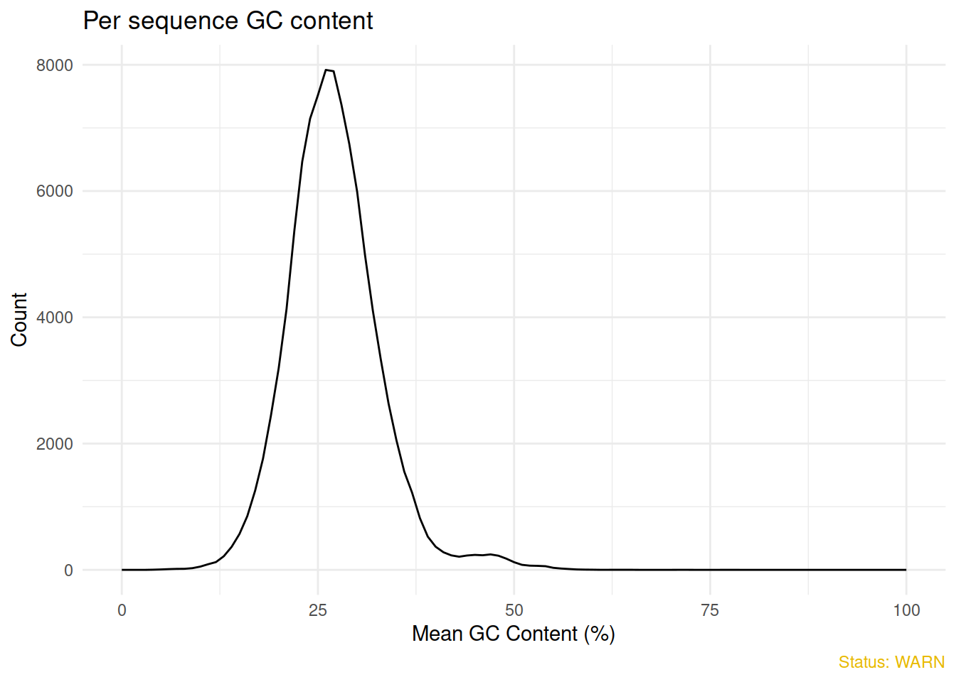

Manipulación de archivos BAM de gran tamaño

Se muestra cómo manejar archivos BAM de gran tamaño ajustando el tamaño de lectura:

yieldSize(bamFile) <- 1
open(bamFile)
scanBam(bamFile)[[1]]$seq
close(bamFile)
yieldSize(bamFile) <- NA

Volver arriba