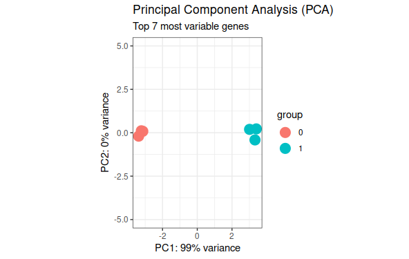
# Convert all samples to rlogddsMat_rlog<-rlog(ddsMat,blind=FALSE)# Plot PCA by column variableplotPCA(ddsMat_rlog,intgroup="Group",ntop=40)+theme_bw()+# remove default ggplot2 themegeom_point(size=5)+# Increase point sizescale_y_continuous(limits=c(-5,5))+# change limits to fix figure dimensions#scale_color_brewer(palette = "Dark2")+ ggtitle(label="Principal Component Analysis (PCA)",subtitle="Top 40 most variable genes")
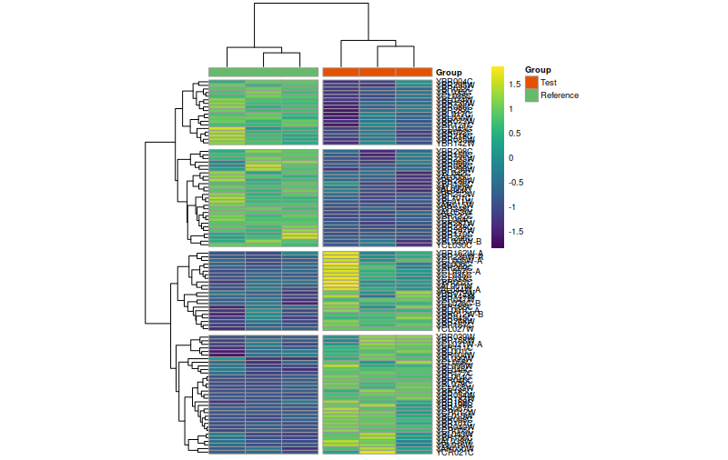
Heatmap de pricipales genes expresados diferencialmente
results_sig<-subset(results,padj<0.05)results_sigddsMat_rlog<-rlog(ddsMat,blind=TRUE)ddsMat_rlogmat<-assay(ddsMat_rlog[row.names(results_sig)])[1:100,]annotation_col=data.frame(Group=colData(ddsMat_rlog)$Group,row.names=colData(ddsMat_rlog)$SampleID)annotation_col$Group<-as.character(annotation_col$Group)annotation_col$Group[annotation_col$Group=="1"]<-"Test"annotation_col$Group[annotation_col$Group=="0"]<-"Reference"ann_colors=list(Group=c("Test"="#E65100","Reference"="#66BB6A"),SampleID=c(a="red"))library(pheatmap)pheatmap(mat=mat,color=viridis(180),scale="row",# Scale genes to Z-score (how many standard deviations)annotation_col=annotation_col,# Add multiple annotations to the samplesannotation_colors=ann_colors,# Change the default colors of the annotationsfontsize=7,# Make fonts smallercellwidth=30,# Make the cells widercutree_cols=2,cutree_rows=4,show_colnames=F)pheatmap(mat=mat,color=viridis(180),scale="row",# Scale genes to Z-score (how many standard deviations)annotation_col=annotation_col,# Add multiple annotations to the samplesannotation_colors=ann_colors,# Change the default colors of the annotationsfontsize=7,# Make fonts smallercellwidth=30,# Make the cells widercutree_cols=3,cutree_rows=4,cluster_cols=F,show_colnames=F)
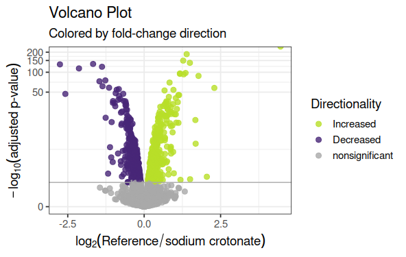
Volcan Plot de genes expresados diferencialmente
data_vp<-data.frame(gene=row.names(results),pval=-log10(results$padj),lfc=results$log2FoldChange)# Remove any rows that have NA as an entrydata_vp<-na.omit(data_vp)library(dplyr)# Color the points which are up or down## If fold-change > 0 and pvalue > 1.3 (Increased significant)## If fold-change < 0 and pvalue > 1.3 (Decreased significant)data_vp<-mutate(data_vp,color=case_when(data_vp$lfc>0&data_vp$pval>1.3~"Increased",data_vp$lfc<0&data_vp$pval>1.3~"Decreased",data_vp$pval<1.3~"nonsignificant"))# Make a basic ggplot2 object with x-y valuesvol<-ggplot(data_vp,aes(x=lfc,y=pval,color=color))# Add ggplot2 layersvol+ggtitle(label="Volcano Plot",subtitle="Colored by fold-change direction")+geom_point(size=2.5,alpha=0.8,na.rm=T)+scale_color_manual(name="Directionality",values=c(Increased="#B8DE29FF",Decreased="#482677FF",nonsignificant="darkgray"))+theme_bw(base_size=14)+# change overall themetheme(legend.position="right")+# change the legendxlab(expression(log[2]("Reference"/"sodium crotonate")))+# Change X-Axis labelylab(expression(-log[10]("adjusted p-value")))+# Change Y-Axis labelgeom_hline(yintercept=1.3,colour="darkgrey")+# Add p-adj value cutoff linescale_y_continuous(trans="log1p")# Scale yaxis due to large p-v
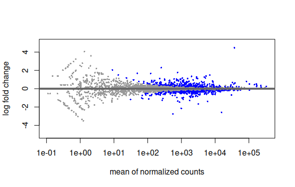
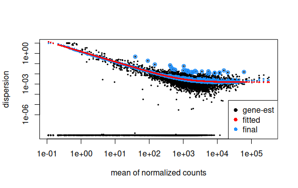
Plot de Dispersion de datos ajustados a modelo de regresión
plotMA(results,ylim=c(-5,5))plotDispEsts(ddsMat)
Análisis de genes especificos
# Convert all samples to rlogddsMat_rlog<-rlog(ddsMat,blind=FALSE)# Get gene with highest expressiontop_gene<-rownames(results)[which.min(results$log2FoldChange)]# Plot single geneplotCounts(dds=ddsMat,gene=top_gene,intgroup="Group",normalized=T,transform=T)